The history of artificial neural networks started in 1961 with the invention of the “Multi-Layer Perceptron” (MLP) by Frank Rosenblatt at Cornell University. Forty years later, neural networks are everywhere: from self-driving cars and internet search engines, to chatbots and automated speech recognition systems.

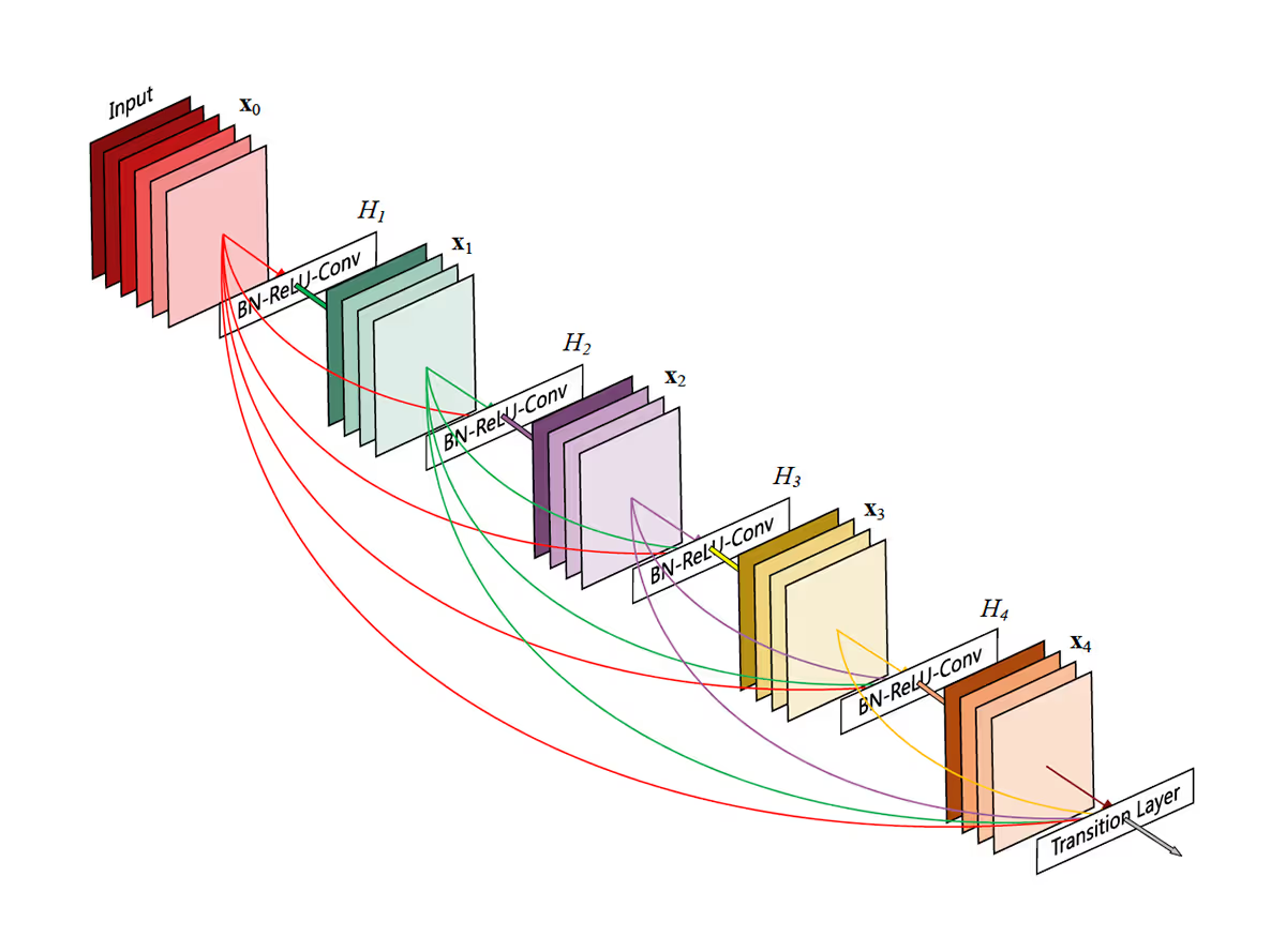
The DenseNet architecture, connects each layer directly with all subsequent layers (of the same size).
Shallow Networks
When Rosenblatt introduced his MLP he was limited by the computational capabilities of his time. The architecture was fairly simple: The neural network had an input layer, followed by a single hidden layer, which fed into the output neuron. In 1989 Kurt Hornik and colleagues from Vienna University of Technology proved that this architecture is a universal approximator, which loosely means that it can learn any function that is sufficiently smooth—provided the hidden layer has enough neurons and the network is trained on enough data. To this day, Hornik’s result is an important milestone in the history of machine learning, but it had some unintended consequences. As multiple layers were computationally expensive to train, and Hornik’s theorem proved that one could learn everything with just a single hidden layer, the community was hesitant to explore deep neural networks.
Deep Networks
Everything changed as cheap GPUs started to proliferate the market. Suddenly matrix multiplications became fast, shrinking the additional overhead of deeper layers. The community soon discovered that multiple hidden layers allow a neural network to learn complicated concepts with surprisingly little data. By feeding the first hiddenlayer’s output into the second, the neural network could “reuse” concepts it learned early-on in different ways. One way to think about this is that the first layer learns to recognize low-level features (e.g. edges, or round shapes in images), whereas the last layer learns high-level abstractions arising from combinations of these low-level features (e.g. “cat”, “dot”). Because the low-level concepts are shared across many examples, the networks can be far more data-efficient than a single hidden layer architecture.
Network Compression
One puzzling aspect about deep neural networks is the sheer number of parameters that it learns. It is puzzling, because one would expect an algorithm with so many parameters to simply overfit, essentially memorizing the training data without the ability to generalize well. However, in practice, this is not what one observed. In fact, quite the opposite. Neural networks excelled at generalization across many tasks. In 2015 my students and I started wondering why that was the case. One hypothesis was that neural networks had millions of parameters but did not utilize them efficiently. In other words, their effective number of parameters could be smaller than their enormous architecture may suggest. To test this hypothesis we came up with an interesting experiment. If it is true that a neural network does not use all those parameters, we should be able to compress it into a much smaller size. Multilayer perceptrons store their parameters in matrices, and so we came up with a way to compress these weight matrices into a small vector, using the “hashing trick.” In our 2015 ICML paper Compressing Neural Networks with the Hashing Trick we showed that neural networks can be compressed to a fraction of their size without any noticeable loss and accuracy. In a fascinating follow-up publication, Song Han et al. showed in 2016 that if this practice is combined with clever compression algorithms one can reduce the size of neural networks even further, which won the ICLR 2016 best paper award and started a network compression craze among the community.

In a nutshell, we forced the network to store similar concepts across neighboring layers by randomly dropping entire layers during the training process. With this method, we could show that by increasing the redundancy we were able to train networks with over 1000 layers and still improve generalization error.
Kilian Weinberger, PhD
Stochastic Depth
Neural network compression has many intriguing applications, ranging from automatic speech recognition on mobile phones to embedded devices. However, the research community was still wondering about the phenomenon of parameter redundancy within neural networks. The success of network compression seemed to suggest that many parameters are redundant, so we were wondering if we could utilize this redundancy to our advantage. The hypothesis was that if redundancy is indeed beneficial to learning deep networks, maybe controlling it would allow us to learn even deeper neural networks. In our 2016 ECCV paper Deep Networks with Stochastic Depth, we came up with a mechanism to increase the redundancy in neural networks. In a nutshell, we forced the network to store similar concepts across neighboring layers by randomly dropping entire layers during the training process. With this method, we could show that by increasing the redundancy we were able to train networks with over 1000 layers and still improve generalization error.
DenseNets
The success of stochastic depth was scientifically intriguing, but as a method, it was a strange algorithm. In some sense, we created extremely deep neural networks (with over 1000 layers) and then made them so ineffective that the network as a whole didn’t overfit. Somehow this seemed like the wrong approach. We started wondering if we could create an architecture that had similarly strong generalization properties but wasn’t as inefficient.

One hypothesis why the increase in redundancy helped so much was that by forcing layers throughout the network to extract similar features, the early low-level features were available even for later layers. Maybe they were still useful when higher-level features are extracted. We, therefore, started experimenting with additional skip connections that would connect any layer to every subsequent layer. The idea was that in this way each layer has access to all the previously extracted features—which has three interesting advantages:
- It allows all layers to use all previously extracted features.
- The gradient flows directly from the loss function to every layer in the network.
- We can substantially reduce the number of parameters in the network.
Our initial results with this architecture were very exciting. We could create much smaller networks than the previous state-of-the-art, ResNets, and even outperform stochastic depth. We refer to this architecture as DenseNets, and the corresponding publication was honored with the 2017 CVPR best paper award.

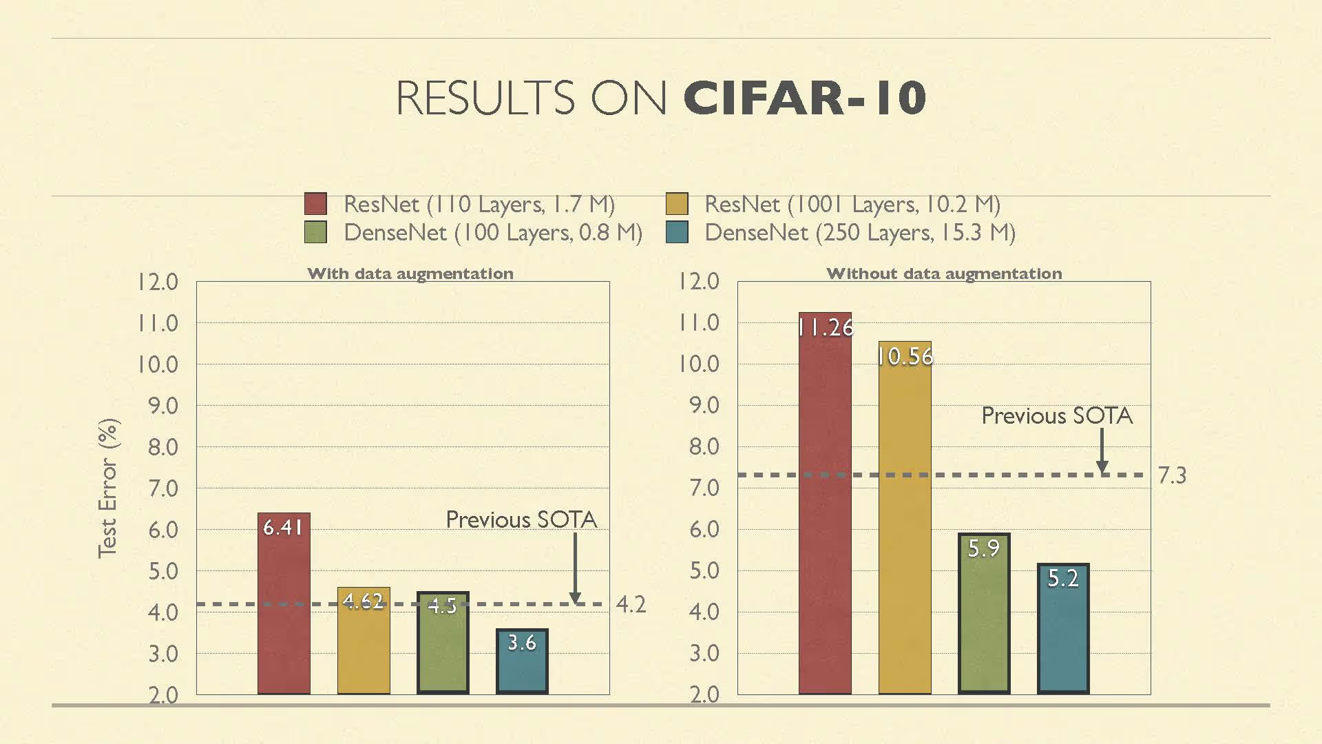
A comparison of the DenseNet and ResNet architecture on CIFAR-10. The DenseNet is more accurate and parameter efficient.
If previous networks could be interpreted as extracting a “state” that is modified and passed on from one layer to the next, DenseNets changed this setup so that each layer has access to all the “knowledge” extracted from all previous layers and adds its own output to this collective state. Instead of copying features from one layer to the next, over and over, the network can use its limited capacity to learn new features. Consequently, DenseNets are far more parameter efficient than previous networks and result in significantly more accurate predictions. For example, on the popular CIFAR-10 benchmark dataset, they almost halved the error rate of ResNets. Most impressively, out-of-the-box, they achieved new record performance on the three most prominent image classification data sets of the time: CIFAR-10, CIFAR-100, and ImageNet.
![(Left:) the chaotic loss landscape of a ResNet 50 with skip connections removed. (Right:) the convex loss landscape of a Densenet 121 (with skip-connections). [Figure from Li et al. 2017]](https://cdn.prod.website-files.com/643d3686e402d4bb8bc58b2e/6459d92197a7dca8e408a2c7_Combine-5.avif)
There may be other benefits from the additional skip connections. In 2017, Li et al. examined the loss surface around the local minimum that neural networks converge to. They found that as networks became deeper, these surfaces became highly non-convex and chaotic—increasing the difficulty to find a local minimum that generalizes beyond the training data. Skip-connections smooth out these surfaces, aiding the optimization process. The exact reasons are still the topic of open research.


